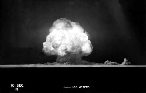
In the late forties not much was known about Manhattan project. The only document that was not kept secret was a film from a Trinity explosion test. The film contained two informations that proved to be valuable in estimating the energy of the wavefront namely time and a length sample. Taylor proposed that the radius of the wavefront is a function of three quantites: energy, time and ρ (density of medium).

r=F(E, t, ρ)

We will now try to give a form of F using ADAM.

Just follow the steps below:

1. If your unit system doesn't contain m, kg, s and N introduce them by using Space definition. (check Define Dimensional Space for details). We will define meter here as an example.
   1. Click space definition in ADAM main window,
   2. In the field symbol write m,
   3. Write meter in the full name field,
   4. Click add.
2. By using the quantites definition window introduce:
   1. r (radius [r]=[m]),
   2. E (energy [E]=[Nm]),
   3. t (time [t]=[s]),
   4. rho (density [rho]=[kg m^-3]) The instruction for defining quantites can be found in the Define Dimensional Space. We will briefly remind them here taking rho as an example:
      1. Click the Define space quantites in the sADAM main window,
      2. Write rho in the symbol field (ADAM doesn't handle greek symbols in a current version!)
      3. Write density in the Description field - this one (as always) is optional,
      4. Write the dimension of a density using multiplication and power operator i.e. kg*m^-3
      5. We won't use tensor description in that example, hence leave those fields at their default. Click Add.
3. Now we shall introduce the postulated dependency r=F(E, t, ρ).
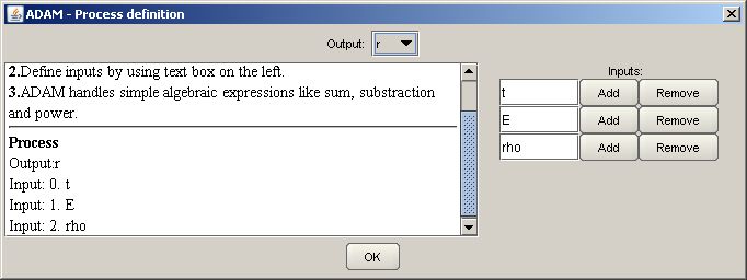
   1. Click the Define process,
   2. In the combo box Output (at the top of the window) choose r,
   3. Enter symbol t in the first Input field,
   4. Then add next input by click add button. Repeat 3. for symbols rho and E,
   5. If everything is ok (confront Ilustration 2) then click OK.
4. Press next once and on the next window click next again (we're not using tensor quantities in that example so that window is of no intrest to us)
5. Check the result. Note that there is only one dimensional base.

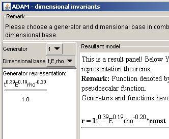
The constant in the formula was obtained by solving an equation of a strong shock wave and appeared to be equal to one.

Now we can estimate the radius of wavefront by using film and a sample length. The time, air density and constant are known and by transformig presented result we can obtain energy of a wavefront. It's simple as that. The same was obtained by Taylor and was a first estimation of wavefront energy outside of Manhattan project and a beutifull application of dimensional analysis as well!

To illustrate the problem let us consider the following example. Point A is rotating with angular velocity &omega₁ along the edge of the disc. The disc itself is in angular motionalong its diameter (Illustration 4). The diameter itself doesn't rotate so the rotation axis stays the same. Without the theory of the process we would state that the resultant acceleration depends on:

a= &Phi (&omega ₁,&omega ₂, r, &rho )

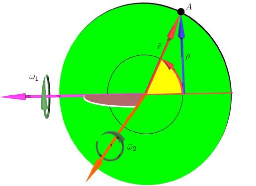
Of course the solution is a sum of three different forces: two centripetal forces and a force coming from Coriolis effect. We will know check if dimensional analysis and Wang theorems can help us derive this result automatically.

Introduce five new quantites:

1. Acceleration a=[m s^-2], vector. To define vector please do the following:
   1. Wirte a and acceleration in fields notation and description respectively (the second one is optional),
   2. In dimension field write m*s^-2,
   3. Now we're changing order of the tensor by choosing second option in the combo box Order. (Order equals to one). Notice that number of element fields has changed.
   4. Leave the Pseudo check box empty (you will use it with angular velocities!),
   5. If everything is ok (confront Ilustration 2) then click OK.
   6. You could change elements fields if you wish but we won't do this in this tutorial. Changing these fields have an important inpact in case of tensors of a second order as ADAM can distinguish between symetric and non symetric matrices.
2. Acceleration omega1=[m s^-1], psuedovector (don't forget to check pseudo check box),
3. Acceleration omega2=[m s^-1], psuedovector (don't forget to check pseudo check box),
4. Position vector r=[m], vector
5. Position vector ro=[m], vector

After defining quantites we guide ourselves ourselves to process definition window. According to mentioned formula we set acceleration a as an ouput quantity and the rest we put to input quantity fields.

We're finished with input data. Let's take a loog at results. Click next in the main window and wait for a second...

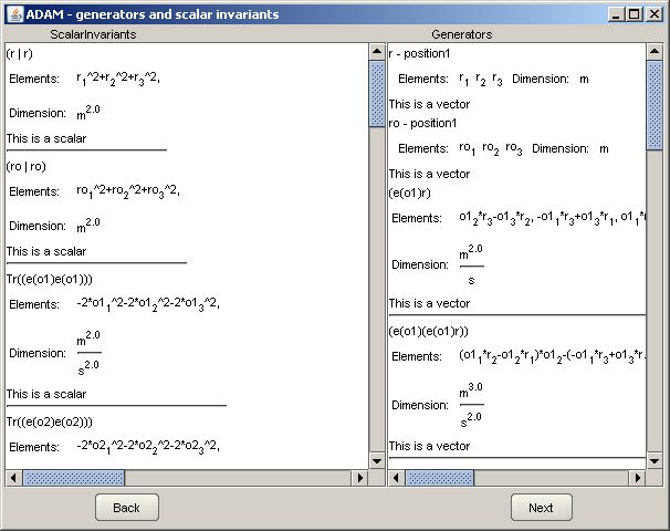
Now you're probably shocked by the amount of generators and scalar invariants. It seams that Wang theorems complicated this simple problem instead of giving straight solution. Bear in mind however that ADAM doesn't know a thing about centripetal and centrifugal forces but still when properly used can recreate intuitive result.

To answer some notational question that may arise now I have to say that e denotes a tensor of a second order accuired from first order pseudo tensor through Levy-Chivita tensor, Tr is a trace and round brackets with a line inside denote scalar product.

To clarify things even further we can note that multiplying two representations of pseudo vectors (which are second order tensors!) with a vector is isomorphic to vector multiplication of three vectors. Let's concentrate on the generators with the same dimension as our output quantity that is m s^-2. Summing up all the remarks we can see that the „right” generators are in that subset. However there are some other generators here as well. So how can we know which generators are „right”? Well that's a hard part here. You have to choose them according to common sense and some other knowledge derived from the problem specific features. Wang and Π theorem are too general give the answer here.